Developing a Linear Regression Algorithm
The Linear Regression is specified as;
where $X_0 = 1$
and;
$(\theta_0, \theta_1, \theta_2,…, \theta_n)$ are the optimized thetas,
$(X_1, X_2,…, X_n)$ are the features or independent variables.
where our algorithm learns from our training data and outputs a prediction hypothesis $h_{(\theta)}(X)$ function which is used to predict actual values of $Y$.
where $\epsilon$ is the Error term.
There are two ways to compute these optimized parameters;
- Gradient Descent
- Normal Equation
A general overview of the process;
- Import required libraries
- Develop model using both Gradient Descent and Normal Equation
- Test Model using both methods on a dataset and compare with Sklearn out-of-the box model using the Root Mean Square Error (RMSE)
Let’s import the important libraries:
import numpy as np
import pandas as pd
from matplotlib import pyplot as plt
from sklearn import datasets
from sklearn.model_selection import train_test_split
from sklearn.metrics import mean_squared_error
1. Gradient Descent
m = Number of Samples
def cost_function(X, y, init0s): #Returns the cost value given the theta values.
  m = len(X) #m is the length of X i.e the number of samples
  cost = 1/(2*m)*np.sum((np.dot(init0s, np.transpose(X)) - y)**2)
  return cost
def partial_derivs(X, y, init0s): #Returns a list of updated thetas
  m = len(X)
  predicted = (np.transpose(init0s) * X).sum(axis = 1)
  diff = (predicted - y)
  diff_transpose = np.transpose(diff[:,np.newaxis])
  #Add a new axis to make it vectorizable for dot product
  updated0s = init0s - alpha*((1/m))* np.dot(diff_transpose, X)[0,:]
  #Remove the extra dimension/axis
  return updated0s
def gradient_descent(X, y,init0s):
  #Returns the optimal theta value and a list of costs for each iteration
  costs = [cost_function(X, y,init0s)]
  for i in range(epochs):
    init0s = partial_derivs(X, y,init0s)
    c = cost_function(X, y, init0s)
    costs.append(c)
  return init0s, costs
def predict(X_test, y_test, optimal0s):
  predicted = (np.transpose(optimal0s) * X_test).sum(axis = 1)
  rmse = mean_squared_error(y_test, predicted)
  return predicted, rmse
Let’s test out our Linear Regression model on a dataset
data = datasets.make_regression(100,2, noise = 1) #100 samples with two features
print(data)
(array([[ 0.0465673 ,  0.80186103],
       [-2.02220122,  0.31563495],
       [-0.38405435, -0.3224172 ],
       [-1.31228341,  0.35054598],
       [-0.88762896, -0.19183555],
       [-1.61577235, -0.03869551],
       [-2.43483776, -0.31011677],
       [ 2.10025514,  0.19091548],
       [-0.50446586, -1.44411381],
       ...
       [-2.06014071,  1.46210794],
       [-0.63699565,  0.05080775],
       [ 1.25286816, -0.75439794],
       [ 1.04444209,  0.81095167],
       [ 1.23616403, -1.85798186],
       [ 2.18697965,  1.0388246 ],
       [-0.07557171,  0.48851815],
       [ 0.59357852,  0.40349164]]), array([  72.36523412,  -37.14156866,  -41.38412368,  -12.64791154,
        -43.66708325,  -55.37682786, -104.14429178,   86.72486169,
       -141.78457722,  -57.09382215,   21.11295519,   37.8001059 ,
        199.5500905 ,   25.81364514,  209.42911479,  128.20604958,
        -26.3460515 ,  -88.2946975 ,   45.84342752,  -29.55352689,
        ...
        102.81595456,  -28.66364244,  100.21268739,  -73.03008828,
       113.01648102,  109.17545836,  -31.30447011,   36.51499677,
       -88.82089559,   -3.4467088 ,   53.45209032,  -87.40808263,
       -99.40016109,    5.04506704,   56.12030581,   84.54855562,
        59.02884225,  -17.38215753,  -24.1274554 ,  102.33610869,
      -120.59599797,  160.11974736,   39.67236875,   55.97220222]))
We need to carry out some preprocessing on data.
- Add the $X_0$ column with 1’s
- Split the data into Train and Split for Validation
def preprocess_data(data):
  X = data[0]
  y = data[1]
  #copy = data.copy
  ones = np.ones(len(X))
  X = np.c_[ones, X]
  return train_test_split(X, y, test_size=0.33, random_state=1)

X_train, X_test, y_train, y_test = preprocess_data(data)
#y_train
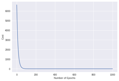
Plot the Cost values
epochs = 1000 #Number of Iterations
alpha = 0.04
init0s = np.zeros(3)

y = gradient_descent(X_train, y_train, init0s)[1]
x = np.arange(len(y))
plt.xlabel("Number of Epochs")
plt.ylabel("Cost")
plt.plot(x,y)
[<matplotlib.lines.Line2D at 0x7f2d50903ac8>]
Optimal Theta Values
gradient_descent(X_train, y_train, init0s)[0]
array([ 0.19357013, 32.19125678, 86.08455637])
So our multivariable linear regression prediction model is;
$h_{(\theta)}(X)$ = 0.19357013$X_0$ + 32.19125678$X_1$ + 86.08455637$X_2$
Compare our model’s RMSE with Sklearn’s
epochs = 1000 #Number of Iterations
alpha = 0.04
init0s = np.zeros(3)
predict(X_test, y_test, gradient_descent(X_train, y_train, init0s)[0])[1]
#Returns the model RMSE
1.4033255546659869
from sklearn.linear_model import LinearRegression
lr = LinearRegression()
lr.fit(X_train, y_train)
prediction = lr.predict(X_test)
rmse = mean_squared_error(y_test, prediction)
rmse
1.4033255545376973
Our model’s RMSE value (1.40332) is comparable to Sklearn’s RMSE value (1.40332)
2. Normal Equation
where $\theta_j = (X^TX)^{-1}X^TY$
def normal_equation(X, y):
  xtrans = np.transpose(X)
  inv = np.linalg.pinv(np.dot(xtrans, X))
  #use pinv for nonivertible singular matrices and use inv for normal invertible matrices
  optimal0s = np.dot(np.dot(inv, xtrans), y)
  return optimal0s
normal_equation(X_train, y_train)
array([ 0.19357013, 32.19125678, 86.08455637])