Regularized Multiclass Logistic Regression Algorithm
A real life example is;
The Logistic Regression is specified as;
where $X_0 = 1$
A key aspect of logistic regression is defining the decision boundary. The decision boundary is delineated by;
Without properly defining the decision boundary, our sigmoid function will output probability values that do not properly classify our sample instances.
A general overview of the process
- Import required libraries
- Develop model using both Gradient Descent
- Test Model using both methods on a dataset and compare with Sklearn out-of-the box model using prediction accuracy
Lets import the important libraries:
import numpy as np
import pandas as pd
from matplotlib import pyplot as plt
from sklearn import datasets
from sklearn.model_selection import train_test_split
Such cost function is stated as;
m = Number of Samples
n = Number of features
def logistic_cost(X_train, y_train, init0s):
  #Returns the cost of our Logistic Regression model given a set of theta parameters (init0s)
  m = len(X_train)
  product = (np.transpose(init0s) * X_train).sum(axis = 1)
  #print(product)
  sigmoid = 1 / (1+ (np.exp(-product)))
  a = (y_train * np.log(sigmoid))
  b = ((1 - y_train) * np.log(1 - sigmoid))
  c = (lambdaa/2*m)*((init0s[1:]**2).sum())
  cost = (-1/m)*np.sum(a+b) + c
  return cost
The goal is to Minimize $J_{(\theta)}$ to output optimized $\theta_j = (\theta_0,\theta_1, \theta_2,…, \theta_n)$ values.
def partial(X_train, y_train, init0s):
  #Returns the partial derivate of the cost function with respect to each theta value
  m = len(X_train)
  prod = (X_train * init0s).sum(axis = 1)
  sigmoid = 1 / (1+ (np.exp(-prod)))
  diff = (sigmoid - y_train)
  update0 = np.asarray(init0s[0] - (alpha/m)*np.dot(diff.transpose(), X_train[:,0]))
  updatej = init0s[1:]*(1 - alpha*(lambdaa/m)) - (alpha/m)*np.dot(diff.transpose(), X_train[:,1:])
  return  np.concatenate([np.expand_dims(update0, axis=0), updatej], axis = 0)
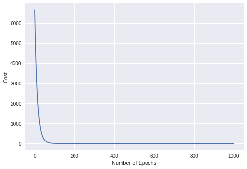
def gradient_descent(X_train, y_train, init0s):
  #Returns the optimal theta value using 3000 iterations
  for i in range(3000):
    init0s = partial(X_train, y_train,init0s)
  return init0s
def oneVsAll(y_array, class_val):
  #Seperates Y into 1's and 0's for each chosen class
  for i in range(len(y_array)):
    if y_array[i] == class_val:
      y_array[i] = 1
    elif y_array[i] != class_val:
      y_array[i] = 0
  return y_array


def multiClassThetas(X_train, y_train, init0s):
  #Returns  a matrix of the optimal theta values with dimension k * n
  #where k is the number of classes and n is number of features
  y_copy = y_train.copy()
  thetas_list = []
  for i in np.unique(y_train):
    copy = y_train.copy()
    y_copy = oneVsAll(copy, i) #Seperate target into 0s and 1s
    class_thetas = gradient_descent(X_train, y_copy, init0s)
    thetas_list.append(class_thetas)
  all_thetas = np.c_[thetas_list]
  return all_thetas
def p_values(thetas, X_train, y_train):
  #Returns each sample instances' probability values for each class with dimension k * m
  #Where k is the number of classes and m is number of samples
  x_tranpose = X_train.transpose()
  p_values = []
  for theta in thetas:
    dot_product = np.dot(theta, x_tranpose)
    p_values.append(1 / (1+ (np.exp(-dot_product))))
  return np.c_[p_values]


def predict(p_values):
  #Returns predictions
  prediction = np.argmax(p_values, axis = 0)
  return prediction

def accuracy_score(prediction, actual):
  #Returns accuracy score (%)
  accuracy_score = sum(prediction == actual) / len(actual)
  return accuracy_score
Let’s test our model on a dataset
digits = datasets.load_digits()
digits
{'DESCR': "Optical Recognition of Handwritten Digits Data...
 'data': array([[ 0.,  0.,  5., ...,  0.,  0.,  0.],
        [ 0.,  0.,  0., ..., 10.,  0.,  0.],
        [ 0.,  0.,  0., ..., 16.,  9.,  0.],
        ...,
        [ 0.,  0.,  1., ...,  6.,  0.,  0.],
        [ 0.,  0.,  2., ..., 12.,  0.,  0.],
        [ 0.,  0., 10., ..., 12.,  1.,  0.]]),
 'images': array([[[ 0.,  0.,  5., ...,  1.,  0.,  0.],
         [ 0.,  0., 13., ..., 15.,  5.,  0.],
         [ 0.,  3., 15., ..., 11.,  8.,  0.],
         ...,
         [ 0.,  4., 11., ..., 12.,  7.,  0.],
         [ 0.,  2., 14., ..., 12.,  0.,  0.],
         [ 0.,  0.,  6., ...,  0.,  0.,  0.]],

        [[ 0.,  0.,  0., ...,  5.,  0.,  0.],
         [ 0.,  0.,  0., ...,  9.,  0.,  0.],
         [ 0.,  0.,  3., ...,  6.,  0.,  0.],
         ...,
         [ 0.,  0.,  1., ...,  6.,  0.,  0.],
         [ 0.,  0.,  1., ...,  6.,  0.,  0.],
         [ 0.,  0.,  0., ..., 10.,  0.,  0.]],


        [[ 0.,  0.,  2., ...,  0.,  0.,  0.],
         [ 0.,  0., 14., ..., 15.,  1.,  0.],
         [ 0.,  4., 16., ..., 16.,  7.,  0.],
         ...,
         [ 0.,  0.,  0., ..., 16.,  2.,  0.],
         [ 0.,  0.,  4., ..., 16.,  2.,  0.],
         [ 0.,  0.,  5., ..., 12.,  0.,  0.]],

        [[ 0.,  0., 10., ...,  1.,  0.,  0.],
         [ 0.,  2., 16., ...,  1.,  0.,  0.],
         [ 0.,  0., 15., ..., 15.,  0.,  0.],
         ...,
         [ 0.,  4., 16., ..., 16.,  6.,  0.],
         [ 0.,  8., 16., ..., 16.,  8.,  0.],
         [ 0.,  1.,  8., ..., 12.,  1.,  0.]]]),
 'target': array([0, 1, 2, ..., 8, 9, 8]),
 'target_names': array([0, 1, 2, 3, 4, 5, 6, 7, 8, 9])}
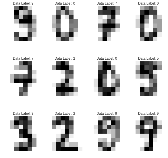
Let’s preview some of the images
#Preview 12 random digits

X = digits["images"]
y = digits["target"]

import random
images_labels = list(zip(X, y))
plt.figure(figsize = (10,10))
for index, (image, label) in enumerate(random.sample(images_labels, 12)):
  plt.subplot(3, 4, index + 1)
  plt.axis('off')
  plt.imshow(image, cmap=plt.cm.gray_r, interpolation='nearest')
  plt.title('Data Label: %i' % label)
We need to carry out some preprocessing on data.
- Add the $X_0$ column with 1’s
- Split the data into Train and Split for Validation
- To apply classification on the images, we need to flatten each image, to turn the data into a (n_samples, feature) matrix
print(digits["images"].shape)
n_samples = len(digits["images"])
data = digits["images"].reshape((n_samples, -1))
print(data.shape)
(1797, 8, 8)
(1797, 64)
def preprocess_data(data,y):
  ones = np.ones(len(data))
  X = np.c_[ones, data]
  return train_test_split(X, y, test_size=0.33, random_state=1)
X_train, X_test, y_train, y_test = preprocess_data(data,y)
X_train.shape
(1203, 65)
Define our parameters
k = set(y_train)
n = X_train.shape[1]
alpha = 0.04
lambdaa = 0.05
init0s = np.zeros(n)
Compute Matrix of Optimal Theta Values
multiClassThetas(X_train, y_train, init0s)
array([[-1.31403414e-02,  0.00000000e+00, -2.59377216e-02,
        -6.31274886e-02,  1.17253991e-02, -6.06195972e-02,
        -2.76216506e-01, -9.60726849e-02, -5.54443559e-03,
        -8.48525208e-05, -1.00972740e-01,  2.88416771e-02,
         1.04467197e-01,  1.07517451e-01,  1.61677709e-01,
        -3.71528350e-02, -6.06298079e-03, -3.37027101e-05,
         5.51556629e-03,  9.99805984e-02, -1.08265132e-02,
        -3.00130630e-01,  2.04669085e-01, -2.50503394e-02,
        -5.75540152e-03,  0.00000000e+00,  5.90709193e-02,
         2.60611419e-02, -1.65867238e-01, -5.10127664e-01,
         3.67345821e-02,  1.94052814e-02, -2.13619661e-03,
         0.00000000e+00,  1.29252327e-01,  1.19501559e-01,
        -2.04148052e-01, -4.83251015e-01, -9.39189012e-02,
         5.43727903e-02,  0.00000000e+00, -4.59732987e-03,
        -9.73487551e-03,  2.18226777e-01, -1.83718565e-01,
        -4.36895134e-01, -2.98278190e-02,  4.10059111e-02,
        -6.33254170e-04, -1.70621937e-02, -7.48627421e-02,
         7.73939584e-02, -7.36453344e-02,  1.00845110e-01,
         1.66573583e-02, -1.53046258e-01, -2.86943181e-02,
        -1.72545249e-05, -2.68832033e-02, -1.40561491e-01,
         1.99166050e-02, -1.11080662e-01, -8.32626265e-02,
        -1.17986780e-01, -2.64299665e-02],
       [-2.69920699e-01,  0.00000000e+00, -1.04710063e-01,
         3.40595678e-01,  3.12234356e-02, -5.64479044e-01,
         3.47876069e-01,  1.12295951e-02, -9.31376715e-02,
        -6.28977921e-04, -6.39244863e-01, -6.02478561e-01,
        -3.31540223e-01,  1.37080523e-02,  2.20134008e-01,
        -3.68506113e-01, -6.10117031e-02, -2.08931048e-04,
         5.06888290e-01,  1.49183942e-01,  4.48823730e-01,
         3.14246111e-01, -3.91285806e-01,  2.12113023e-01,
        -6.55962009e-03,  0.00000000e+00, -2.74605434e-01,
         3.75841347e-02,  1.42843851e-01, -1.04040246e-02,
         9.69674873e-02, -2.23627666e-01, -9.41148407e-05,
         0.00000000e+00,  1.37636303e-02, -9.77820381e-03,
        -3.65732736e-01,  2.80348134e-01, -9.46361310e-02,
        -3.88469464e-01,  0.00000000e+00, -1.94733356e-03,
        -6.18295375e-01,  5.00341696e-02,  1.19085853e-01,
        -9.93209820e-02, -1.65864730e-01, -2.53260827e-01,
        -5.71349313e-03, -1.12283576e-02, -2.59447562e-01,
        -4.69374156e-02,  1.37028882e-01,  9.03339949e-02,
        -1.02199302e-01, -2.68638669e-01,  3.93152618e-01,
        -3.60629707e-03, -2.03306602e-01, -3.15610518e-01,
        -1.29422171e-02,  7.87461417e-02,  1.87173583e-01,
        -2.86360508e-01,  2.73121918e-01],
        ...
Compute Probability values using optimal thetas on the Test set
optimal_thetas = multiClassThetas(X_train, y_train, init0s)
p_values(optimal_thetas, X_test, y_test)
array([[1.30693813e-10, 5.47023277e-05, 9.99988296e-01, ...,
        5.69104368e-12, 2.71614471e-09, 9.99978225e-01],
       [9.50544243e-01, 6.62287815e-08, 2.03516481e-10, ...,
        5.34710312e-11, 2.22894272e-04, 9.88195491e-08],
       [1.71002761e-06, 2.92223351e-05, 3.23123282e-06, ...,
        7.73583827e-06, 7.06966327e-16, 4.44882769e-06],
       ...,
       [1.67917238e-06, 6.32334394e-02, 2.18410678e-07, ...,
        1.03953150e-06, 2.22179681e-06, 8.15802069e-07],
       [4.96943926e-03, 3.67007637e-05, 4.79761046e-11, ...,
        6.25440616e-01, 3.62788141e-07, 1.79991157e-07],
       [4.16670602e-07, 3.59481313e-05, 6.75722211e-08, ...,
        1.77055305e-06, 3.09914373e-05, 1.89162455e-07]])
Compute Test Predictions
prob = p_values(optimal_thetas, X_test, y_test)
predict(prob, y_test)
array([1, 5, 0, 7, 1, 0, 6, 1, 5, 4, 9, 2, 7, 8, 4, 6, 9, 3, 7, 4, 7, 4,
       8, 6, 0, 9, 6, 1, 3, 7, 5, 9, 8, 3, 2, 8, 8, 1, 1, 0, 7, 9, 0, 0,
       8, 7, 2, 7, 4, 3, 4, 3, 4, 0, 4, 7, 0, 5, 9, 5, 2, 1, 7, 0, 5, 1,
       8, 3, 3, 4, 0, 3, 7, 4, 3, 4, 2, 9, 7, 3, 2, 5, 3, 4, 1, 5, 5, 2,
       5, 2, 2, 2, 2, 7, 0, 8, 1, 7, 4, 2, 3, 8, 2, 3, 3, 0, 2, 9, 5, 2,
       3, 2, 8, 1, 1, 9, 1, 2, 0, 4, 8, 5, 4, 4, 7, 6, 7, 6, 6, 1, 7, 5,
       6, 3, 8, 3, 7, 1, 8, 5, 3, 4, 7, 8, 5, 0, 6, 0, 6, 3, 7, 6, 5, 6,
       2, 2, 2, 3, 0, 7, 6, 5, 6, 4, 1, 0, 6, 0, 6, 4, 0, 9, 3, 5, 1, 2,
       3, 1, 9, 0, 7, 6, 2, 9, 3, 5, 3, 4, 6, 3, 3, 7, 4, 8, 2, 7, 6, 1,
       6, 8, 4, 0, 3, 1, 0, 9, 9, 9, 4, 1, 8, 6, 8, 0, 9, 5, 9, 8, 2, 3,
       5, 3, 0, 8, 7, 4, 0, 3, 3, 3, 6, 3, 3, 2, 9, 1, 6, 9, 0, 4, 2, 2,
       7, 9, 1, 6, 7, 6, 5, 9, 1, 9, 3, 4, 0, 6, 4, 8, 5, 3, 6, 3, 1, 4,
       0, 4, 4, 8, 7, 9, 1, 5, 2, 7, 0, 9, 0, 4, 4, 0, 1, 4, 6, 4, 2, 8,
       5, 0, 2, 6, 0, 1, 8, 2, 0, 9, 5, 6, 2, 0, 5, 0, 9, 1, 4, 7, 1, 7,
       0, 6, 6, 8, 0, 2, 2, 6, 9, 9, 7, 5, 1, 7, 6, 4, 6, 1, 9, 4, 7, 1,
       3, 7, 8, 1, 6, 9, 8, 3, 2, 4, 8, 7, 5, 5, 6, 9, 9, 9, 5, 0, 0, 4,
       9, 3, 0, 4, 9, 4, 2, 5, 4, 9, 6, 4, 2, 6, 0, 0, 5, 6, 7, 1, 9, 2,
       5, 1, 5, 9, 8, 7, 7, 0, 6, 9, 3, 1, 9, 3, 9, 8, 7, 0, 2, 3, 9, 9,
       2, 8, 1, 9, 8, 3, 0, 0, 7, 3, 8, 7, 9, 9, 7, 1, 0, 4, 5, 4, 1, 7,
       3, 6, 5, 4, 9, 0, 5, 9, 1, 4, 5, 0, 4, 3, 4, 2, 3, 9, 0, 8, 7, 8,
       6, 9, 4, 5, 7, 8, 3, 7, 8, 3, 2, 6, 6, 7, 1, 0, 8, 4, 8, 9, 5, 4,
       8, 2, 5, 3, 3, 3, 5, 1, 8, 7, 6, 2, 3, 6, 2, 5, 2, 6, 4, 5, 4, 4,
       9, 7, 9, 1, 0, 2, 6, 9, 3, 6, 7, 3, 6, 4, 7, 8, 4, 1, 2, 1, 1, 0,
       7, 3, 0, 3, 2, 9, 4, 5, 9, 9, 4, 8, 3, 3, 3, 8, 4, 1, 4, 5, 8, 3,
       9, 5, 4, 7, 7, 4, 0, 1, 7, 9, 8, 0, 9, 6, 0, 9, 8, 6, 3, 1, 4, 6,
       5, 1, 9, 0, 1, 5, 2, 5, 0, 2, 5, 4, 7, 2, 2, 3, 2, 1, 8, 4, 9, 6,
       3, 7, 1, 1, 1, 8, 8, 8, 8, 5, 9, 1, 7, 1, 2, 7, 9, 7, 4, 3, 4, 0])
Check for Accuracy
prediction = predict(prob)
accuracy_score(prediction, y_test)
0.9696969696969697
Compare With Sklearn’s Logistic Regression Module
from sklearn.linear_model import LogisticRegression
lr = LogisticRegression()
lr.fit(X_train, y_train)
accuracy_score(y_test, lr.predict(X_test))
0.9562289562289562
Our model’s accuracy score on the Test set is 96.96% which is better than Sklearn’s 95.6%
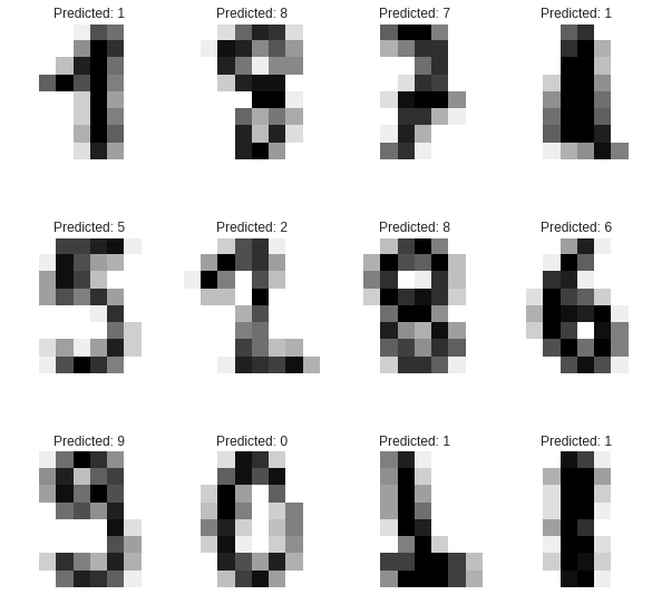
Let’s check the performance of our model visually. To do this, we have to remove the $X_0$ (1) values and reshape to shape (n_samples, 8, 8)
X_test_reshaped = X_test[:,1:].reshape(len(X_test), 8, 8)
X_test_reshaped.shape
(594, 8, 8)
images_prediction = list(zip(X_test_reshaped, prediction))
plt.figure(figsize = (10,10))
for index, (image, prediction) in enumerate(random.sample(images_labels, 12)):
  plt.subplot(3, 4, index + 1)
  plt.axis('off')
  plt.imshow(image, cmap=plt.cm.gray_r, interpolation='nearest')
  plt.title('Predicted: %i' % prediction)